Formation of Double-Diffusive Intrusions

This page provides access to a recording of double-diffusive intrusion formation in a stable salt-stratified liquid. I created the recording shortly after my Ph.D. defense, for a scientific committee demonstration. To this end I perfomed three simulations with different Rayleigh number and buoyancy ratio, and used snapshots as frames for a movie. Subsequently I put the movie on videotape.

Nowadays the internet is the common way to distribute information, and since the videotape began to show slight signs of deteroriation I decided to release a digital version. As I did not have access to the original code anymore I took the video recordings as the source after some "cleaning up"

The video relates to Chapter 3 of my thesis, and I refer to that part for a detailed model and results description.

Simulation design: relation between physics, scaling and discretization

Since computational resources are always limited it is important to take into account as much information of the physics involved as possible when designing a numerical simulation experiment, i.e. defining the proper scaling (for making the equations non-dimensional) and the proper parameter definitions. In this type of "diffusive-mode" double-diffusive convection this means that we take into account the layer thickness scale h , the Rayleigh number based on this lengthscale scale, Ra_h , and the buoyancy ratio R.

To cast the model equations in dimensionless form I scaled variables in such a way that the relation between the layer thickness h and the container physical (i.e. dimensional) height H is given by h = H/R, i.e. we may expect approximately R convection cells. Thus we are "in control" numerically; by keeping R relatively low proper numerical resolution of the thin boundary layers and diffusive interfaces can be obtained (but at the expense of some influence of the upper and lower horizontal container boundaries). Note also that for fixed R the effect of increasing Ra_h is to effectively increase the physical domain geometry for a given set of boundary conditions.

What is shown?

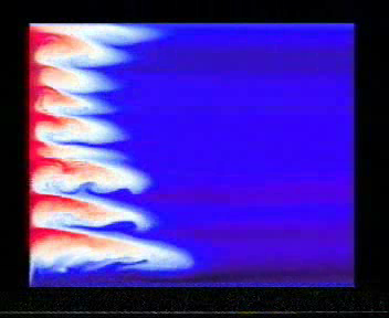
The movie shows the perturbation of a stable, salt-stratified initially motionless column of water by suddenly applying and maintaining a temperature jump with respect to the initial uniform temperature at the left sidewall. Shown is the perturbation of the initial linear salinity gradient, effectively causing salt to be used as a tracer. Using the perturbation instead of the salt concentration itself results in much more detail being visible, particularly within the convective layers. A red color denotes an increase of salinity with respect to the initial gradient, blue implies a decrease. Note that the coloring scheme used does not indicate temperature!

Experiment 1

Weak buoyant forcing (Ra_h = 5*10⁴), low buoyancy ratio (R = 2.5)

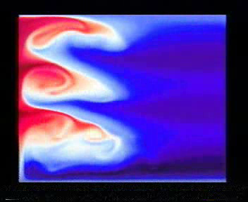
The first simulation shows the formation of relatively weak convection cells in which only partial mixing occurs; many details remain visisble in the cells during the evolution of the flow. The simulation clearly reveals that the magnitude of the convective motion within the cells is much larger than the propagation speed of the front of the layered system

Experiment 2

Weak buoyant forcing (Ra_h = 5*10⁴), high buoyancy ratio (R = 5)

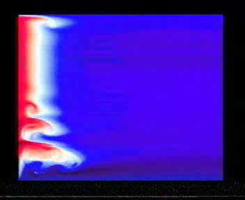
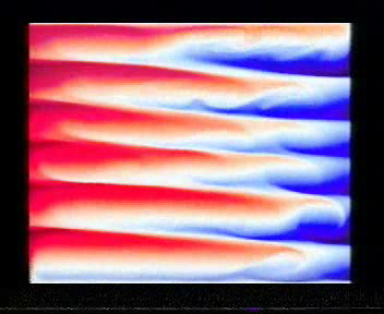
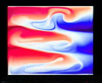
The second simulations reveals various interesting features:

- In the initial phase instabilities propagate along the unstable initial boundary layer from the bottom, and some initial convection cells quickly get overwhelmed by neighboring cells.

- In the two convective layers in the center of the container mixing occurs through secondary instabilities which cause weak but persistent clock-wise rotating convection cells to emerge. These cells are most likely caused by the instability mechanisms as investigated and described by Kerr.

- The layer development causes the density distribution in the fluid to the right of it to be modified as well.

Experiment 3

Strong buoyant forcing (Ra_h = 2*10⁵), high buoyancy ratio (R = 5)

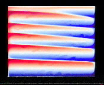
- A characteristic of the third experiment is the occurrence of layer merging on two timescales: Like in experiment 2 some of the initial convection cells get rapidly consumed by stronger neighboring ones, but this simulation also shows that layer merging occurs much later when the layers already have developed; one layer gets slowly 'sandwidched'. This process is decsribed in detail in Chapter 3 of my thesis.

- This simulation also shows a much more vigorous convection process, with instabilities occuring along the initial thermal boundary layer almost simultaneously. As a result the convective layers are well mixed and have an almost uniform salt distribution.

- The layer structure appears to be remarkably stable after merging. Still further merging might have happened if the simulation had been proceeded.

Movie Download

Please download the movie locally by right-clicking on the following link

Contact: jurjen CURLY_A kranenborg PUNKT org